When it comes to successfully managing spreadsheets, accuracy is essential. One important thing you can do to make your Excel work more accessible is to delete filtered rows. This involves eliminating unnecessary rows of data from your spreadsheet, which helps you manage it more effectively.
When dealing with a large amount of information or trying to organize it, it can be helpful to know how to achieve this. In this simple article, we’ll explain each step in detail, so you quickly understand how to use Excel’s filtering capabilities and improve your data organization.
Understanding Excel Filters
Before removing anything, you must know how Excel’s filters function. Filters are like magical tools that display only the information you want. They hide all the rows that don’t match the rules you set. Filters are super helpful when figuring out important stuff from big data.
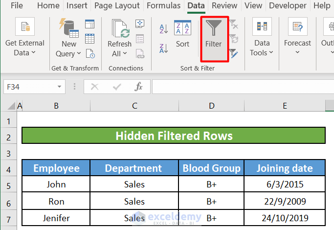
To apply a filter in Excel, first choose the cells containing your data. Then, select the “Data” tab at the top of the display. The filter button shows as a funnel-shaped button. Your data is now ready to be filtered. You’ll see little arrows next to each column’s name – the filters are on.
Filtering Your Data
Once you turn on the filters, you’re in control. You can change how you see your data by setting rules for each column. Just click on the little arrow at the top of the column you want to filter and pick what you want to see. Excel offers many filtering options, including words, numbers, and dates.
For example, if you’re interested in sales data, you may filter the “Sales” column to only show values more significant than a particular number or from a specific time frame. It lets you focus on the details you need, making it easy to comprehend and make decisions.
Delete Filtered Rows
Deleting filtered rows in Excel is a process that involves removing specific rows of data based on applied filter criteria. This function is handy when cleaning up your dataset by eliminating unnecessary or irrelevant information. Here’s a detailed explanation of how to delete filtered rows in Excel:
Apply Filters
First, before removing rows, you have to set up your filters. It’s like setting on special glasses that allow you to notice what you want to see. To do this, select the cells where your data lives and lead to the “Data” tab at the top of the screen. Look for the “Filter” button and click it.
You’ll see little indicators following each column, meaning your filters are ready to go. Now, you’re all set to begin cleaning up your spreadsheet.

Filter Data
After you’ve set up your filters, it’s duration to get particular about what you see. You can change how your data looks by setting up rules for each column. Click on the small arrow at the lid of the column you want to change and pick what you want to see.
Excel offers multiple options, like sorting by words, numbers, or dates. This way, you can zoom in on the stuff you need, making it easier to understand and work with your data.

Select Filtered Rows
Once you’ve set up your filters, Excel shows only the rows that match your rules, hiding the rest out of sight. Now, if you want to delete those filtered rows, here’s what you do: start by picking them out. Click on any cell within the filtered data, then hit Ctrl + A on your keyboard.
That shortcut grabs all the cells you can see in the filtered range, leaving out any hidden ones. You’re ready to tidy up your spreadsheet and remove those unwanted rows.

Delete Rows
Once you’ve set the rows you want to eliminate, it’s time to say goodbye to them. To do this, right-click anywhere in the assigned area and look for the “Delete” option in the pop-up menu. You can push the “Delete” key on your keyboard if you choose shortcuts.
Excel will then double-check with you to make sure you want to delete those rows, avoid accidents, and maintain your data safe. Once you confirm, those filtered rows will vanish from your spreadsheet, leaving it nice and tidy.

Review Changes
Once you’ve said goodbye to the filtered rows, giving your spreadsheet a quick once-over is a good idea. Please take a moment to delete filtered rows excel it and ensure everything looks right. Check if the rows you wanted to delete are gone and your data still makes sense. You want to make sure that nothing important got deleted by mistake. This extra step can help you catch errors and keep your spreadsheet in tip-top shape.

Undo Deletion (Optional)
If you suddenly recognize you made a mistake and deleted the incorrect rows, don’t worry. Excel has got your back with its convenient undo feature. Just press Ctrl + Z on your keyboard, or look for the “Undo” control on the toolbar and give it a click. This magical button lets you shift back time and undo your last action, including deleting those rows. So, if you are required to return something you accidentally fired, just hit that undo control and watch as Excel works its magic to restore your data.
Using these instructions to delete filtered rows excel, you may successfully erase purified rows in Excel, optimize your data management method, and confirm that your spreadsheet only has the report required for research and reporting.
How to Delete Visible Filter Rows in Excel using Go To Special
To delete visible filter rows in Excel using “Go To Special,” follow these steps:
1. Apply Filter: Start by filtering your data range. It can be done by setting the range of cells with your data and then clicking on the “Filter” button in the “Data” tab of the Excel stripe.
2. Select Visible Cells: With the Filter applied, you’ll see only the rows that meet the filter indicator. Now, select the entire range of visible cells you want to delete.

3. Go To Special: To open the Go To Special, use the keyboard shortcut Ctrl + G to activate the Go To dialog box. Additionally, go to the Home tab click the Find & Select drop menu, and choose Go To Special.

4. Select Visible Cells Option: In the “Go To Special” text box, select “Visible cells only” and click “OK.” It will only choose the visible cells in the range, leaving out hidden ones.

5. Delete selected Rows: Once the visible cells have been chosen, press the Delete key on your keyboard to remove them. You can also right-click on the chosen cells and choose Delete from the context menu.

6. Confirm Deletion: Excel will remind you to verify the Deletion. Click “OK” to proceed.

Following these steps, you can quickly delete visible filter rows in Excel using the “Go To Special” feature. This method lets you promptly remove filtered data while retaining hidden rows that do not meet the filter criteria.
Conclusion
Learning to delete filtered rows in Excel is a helpful skill that can significantly improve productivity and facilitate your data management workflow. Understanding Excel’s filtering features and following the step-by-step guide.
In this manual will allow you to efficiently clean your spreadsheets and concentrate on the most crucial data. Incorporate these tactics into your Excel repertoire and watch as your productivity increases.
FAQs
Will deleting filtered rows also remove the filter in Excel?
No, deleting filtered rows does not automatically remove the filter. The filter will remain active, but the deleted rows will be removed from the dataset.
Can I undo the deletion of filtered rows in Excel if I make a mistake?
Yes, you can use the undo segment in Excel (Ctrl + Z) to regress the deletion of filtered rows if you accidentally remove the incorrect data.
Does deleting filtered rows affect the rest of my Excel spreadsheet?
Deleting filtered rows removes the selected rows from your dataset and does not impact other data in your spreadsheet.
Is there a fast way to delete filtered rows in Excel without manually selecting them?
Yes, you can use Excel's "Go To Special" feature to fast select and delete only the filtered rows, saving duration and struggle.


